Clean up your data
Learn how to clean up data in Microsoft Excel 2010
Introduction (00:04)
Welcome to Business Productivity – I’m Ulrika Hedlund. From time to time you are given a data file that you need to clean up in order to make some sense of it. The data might have been extracted from a database in which case it isn’t very user friendly to read. If you’re working with large sets of data you don’t want to waste your time by manually going through a large set of rows and columns.
Microsoft Excel 2010 is a great tool for cleaning up large sets of data, and if you learn the techniques and shortcuts you can quickly arrange the data in a format that makes sense to you.
In this video I will show you how you can take a spreadsheet and how you can clean it up by changing the layout, deleting unwanted data and spotting and removing duplicates. Let me show you!
Changing column and row size (01:00)
Here I have an email from a colleague with two files attached. These are Excel files with data that has been extracted from a database. The files contain information about prospects that we are going to share with an agency for analysis. I’m going to save these attachments to a document library and then I want to consolidate them into one single spreadsheet and clean up the data.
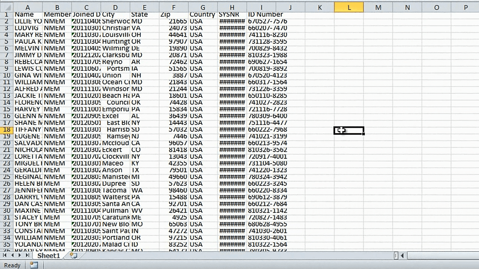
Let’s start by opening up the first spreadsheet. As you can see it’s quite difficult to read this data.
One of the columns seems to contain only hash tag symbols. This is Excel’s way of telling you that the contents in this column can’t fit the current width of the cell. To see the full content I can either drag the column to the right by holding down the left mouse button, or I can just double click to the right of the column.
Instead of resizing individual columns I can resize all columns and rows at the same time. To do that, mark the entire spreadsheet and then double click between two columns or two rows.
The entire spreadsheet is now a lot easier to read. I also want to make the column headings stand out a bit more so I’ll mark the first row and make it bold.
Turning data from row to column (transposing data) (02:20)
Now I’ll open up the other spreadsheet with data. Again, I’ll mark the entire spreadsheet and increase the column width. As you can see, I have the same type of prospect information in this file, but the data is rotated the other way. Since I want to have all the data in one single spreadsheet, I’ll mark this data, right-click and copy it. Now I’ll go back to my first spreadsheet where I want to append this data. To go to the very end I’ll press CTRL+ End. This takes me to the last cell. Now I’ll mark the first empty cell where I want the data to be copied, I’ll right click and under “Paste Options” I’ll select to “Transpose” the data.
The data is copied and turned to match the layout of this data. To go back to the top row again I’ll press CTRL + Home.
Deleting and moving columns (03:17)
Now that I have all my data in one spreadsheet I want to delete some unnecessary data and change the order a bit. I don’t need this “System Number” column so I’ll mark it by left-clicking on the column letter, right-click and select “Delete”.
Now I want this “ID Number” column which has unique values for each individual to be the very first column. I’ll move my mouse cursor to either side of the column until I see a cross, then I’ll hold down the right mouse button and drag the column to the desired position.
From the menu I’ll select “Shift Right and Move”. The columns are shifted to the right to make room for the ID Number column.
I’ll also mark the Address and Country columns and move them to the right of the Name column, again selecting to shift and move the data that is currently there.
Spotting and highlighting duplicates (04:15)
When you’re working with a large set of data, it’s difficult to see if you have duplicates. If you easier want to spot duplicates you can sort and color duplicate data. Here I’ll choose to sort by name by clicking a cell in the Name column, then I’ll go to the “Data” tab and click the “A-Z” button. Now the names are sorted alphabetically, and it’s easier to notice duplicate names.
To make it even easier I’ll choose to color duplicates. I’ll go back to the Home tab, then I’ll mark the entire range of names by holding down the (CTRL and) Shift key and then pressing arrow down.
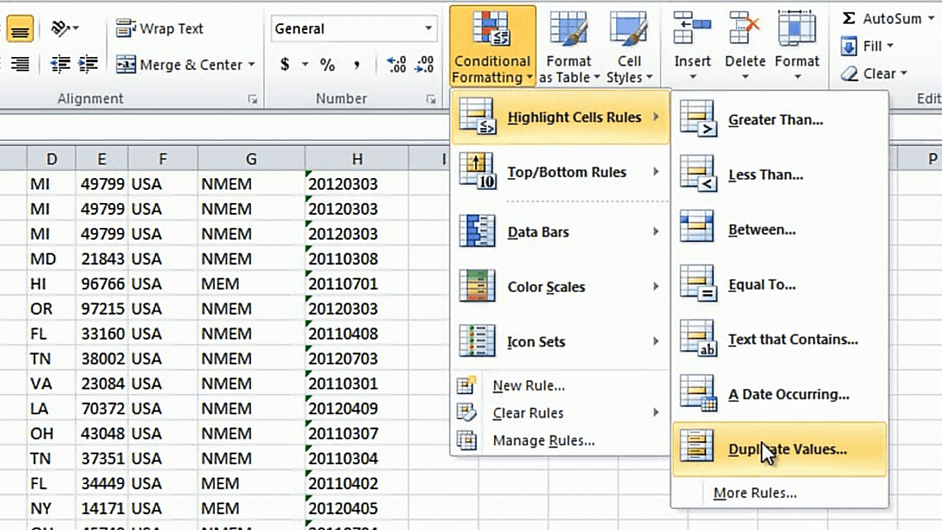
Under the Styles Group, I’ll click “Conditional formatting” and select “Highlight Cells Rules”, I’ll click “Duplicate Values” and leave the default coloring which is light red fill with dark red text.
Now I can easily see names that are duplicates. As you can see these entire records are identical, but in some cases two people might have the same name. If I scroll down here you can see that I have two “Andre Bishop” with the same name, but different ID numbers.
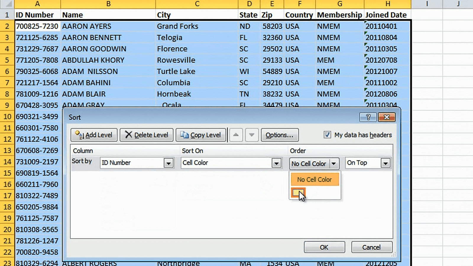
In this case it’s better to look for duplicates in the ID number column. I’ll mark the entire range of ID numbers by holding down the (CTRL and) Shift key while I press arrow down. I’ll click “Conditional Formatting”, “Highlight Cells Rules”, “Duplicate Values”, and here I’ll change to a yellow color formatting. Now I want to sort the ID Number column by color. I’ll go to the “Data” tab again and click the “Sort” button. Here I’ll select to sort by ID number and sort on cell color and I’ll choose to have the colored cells on top.
Now it’s really easy for me to see all the duplicate records.
Using Excel to automatically remove duplicates (06:15)
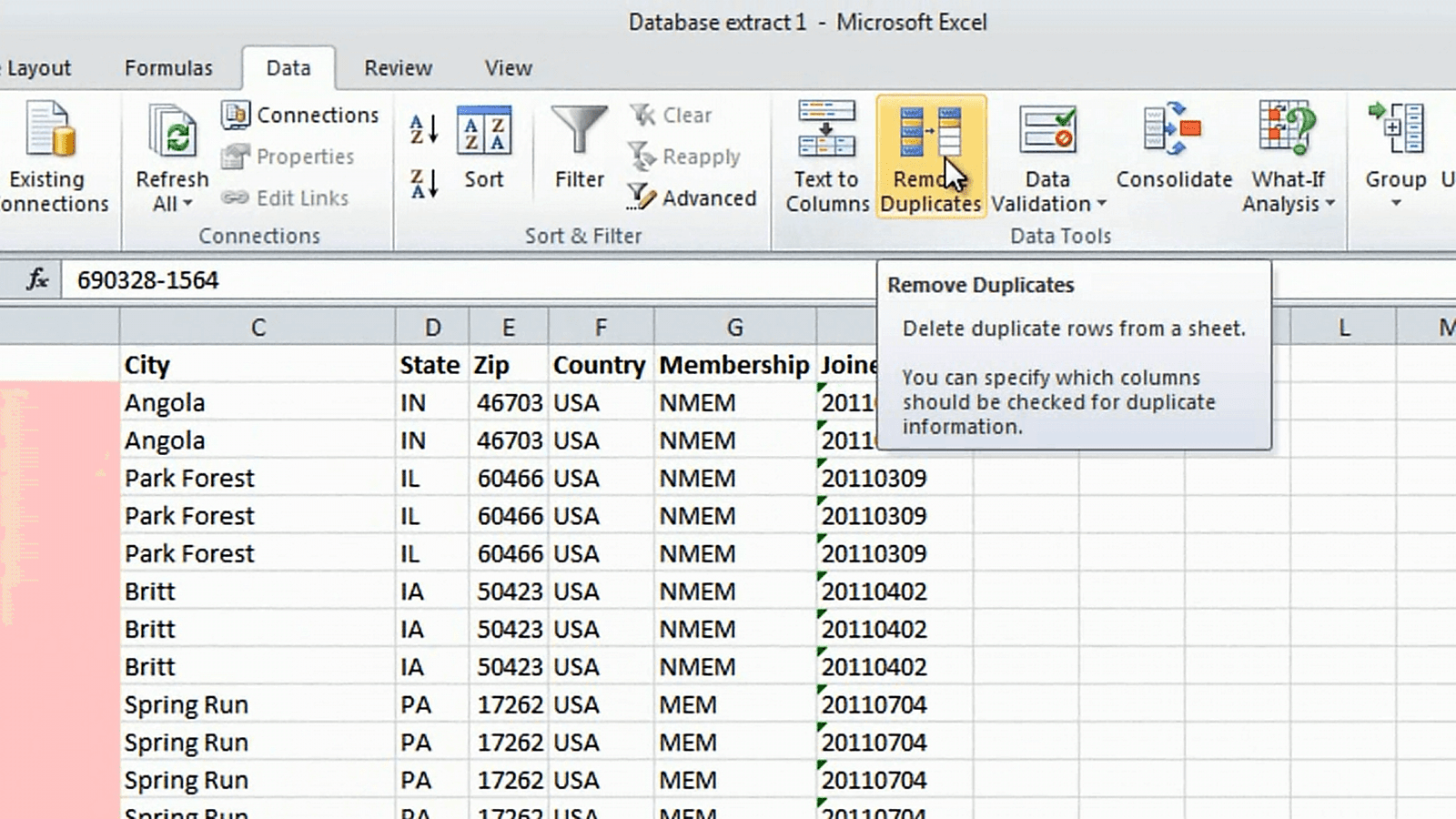
However, instead of manually deleting duplicates I can use a built in tool in Excel to remove duplicates. On the “Data” tab in the “Data Tools” section I’ll click “Remove Duplicates”.
I’ll leave the check box that says “My data has headers” marked and I’ll also leave all the columns checked since I only want to remove rows where the values in all the columns are the same, and then I’ll click “Ok”. Now as you can see, Excel removed 45 duplicate values for me. All the duplicate ID numbers have now disappeared just like we wanted, but the red coloring in the name column tells us that we still have some duplicate names. This is fine since we have different people with the same name.
Remove conditional formatting (07:03)
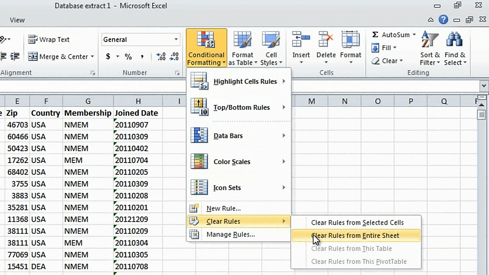
To remove the red coloring of the name I’ll click the “Home” tab and under the “Styles” group I’ll click “Conditional Formatting” again, I’ll select “Clear Rules” and then “Clear Rules from Entire Spreadsheet”.
Now I’ve cleaned up my data so that it’s easier for me to manipulate and analyze.
Closing (07:23)
The spreadsheet that I used here had a little over one thousand rows of data. In many scenarios you will be working with a lot larger data sets. By using the techniques I showed you in this video it will be much easier for you to clean up your data. In the video called “Modify and manipulate data” I’ll show you how you can go deeper with Excel 2010 to modify your data. I’m Ulrika Hedlund for Business Productivity – thanks for watching!


