
Modify and manipulate data
Learn how to modify and manipulate data using Microsoft Excel 2010
Introduction (00:04)
Welcome to Business Productivity – I’m Ulrika Hedlund. Quite often you have a spreadsheet with data that you want to manipulate in some way. You might want to share the data with others but before you do, you need to modify, remove or censor some of the data. Microsoft Excel 2010 has a lot of built in functions that you can use to manipulate data, but if you don’t use these frequently they’re very easy to forget so you might end up doing things manually instead.
In the video called “Clean up your data” I show you how you can use Microsoft Excel 2010 to clean up large data sets. In this video I’ll show you how you can manipulate data by combining and splitting columns, by censoring data and also by changing data types. Let me show you!
Changing from upper case to lower case (00:58)
Here I have data extracted from a database that I want to modify so that it’s easier to work with. First I want to change the “Name” column so that the letters aren’t all upper case. I also want to add an additional column for first name and last name. I’ll start by adding two new empty columns to the right. To do that I’ll right-click on the column to the right and select “Insert”, I’ll do it one more time to add an additional column. I’ll change the name of this column from “Name” to “Full Name”. To find a function to make only the first letter upper case I’ll go to the “Formulas” tab and select “Insert function”.

I’ll write a description of what I want to do “first letter uppercase”. Here Excel lists some options. The second one called “PROPER” sounds right “Converts a text string to proper case”. I’ll insert the function and select the text I want to convert and then click “Ok”.

You can see that the name “Allen Gibbs” was converted correctly. To copy this formula for the entire range of cells I’ll just double click the little cross in the bottom right corner. Great! Now all the names have been converted. Now I want to replace the original content with this converted text. I’ll right-click and drag the new content over the “Full Name” column and select “Copy here as Values Only”.

This means that the formula I used will be removed and only the name itself will be copied over. I’ll clear the contents in this column by right-clicking and selecting “Clear Contents”.
Splitting a column into two (02:38)
Now I’ll add headings for the new columns, “First Name” and “Last Name”. Then I’ll mark the contents of the entire “Full Name” column by clicking on the first cell and then pressing CTRL-Shift and then arrow down on the keyboard. I’ll go to the “Data” tab and click “Text to columns”.

This wizard will help me split the full name into first name and last name. In the first step I need to state the data type, I’ll leave the first option which is “Delimited”, and click “Next”. Here I need to tell the wizard how the first names and last names are separated; I’ll uncheck “Tab” and select the checkbox for “Space”. I get a preview of the data here so that I can see what the end result will look like.

I’ll click “Next” again to go to the final step. Here I need to enter the destination for the names. I’ll mark the first cell in the range and then click “Finish”. Now you can see that I have the two columns filled with “First” and “Last Name”.
Removing unnecessary spaces (03:36)
Now let’s have a look at the “City” column. By just looking at it I can see that there are some leading spaces here.

This becomes very apparent if you sort on this column. As you can see Excel first sorts the city names that start with a space and then the rest. This is not the way I want the data so I want to remove these spaces. I’ll insert a temporary empty column by right-clicking and selecting “Insert”, and then I’ll go back to the “Formulas” tab and click “Insert function”, again I’ll write a short description “Clear spaces.” Here Excel suggests a function called “TRIM” which removes unnecessary spaces.

I’ll mark the first cell in the “City” column and click “OK”. Again I’ll copy the formula by double-clicking in the bottom right corner. I’ll right-click and drag the content over, and select “Copy Here as Values Only”. Then I’ll remove the temporary column by right-clicking and selecting “Delete”. Now I want to sort this column again, so I’ll go to the “Data” tab and click sort “A-Z” and now the city names are sorted properly.
Combining data from multiple columns into one (04:45)
Now I want to combine data from the three columns “City”, “State” and “Zip” code into one column called “Address”. First I’ll insert a new column that I name “Address”, then I’ll go to the “Formulas” tab, click “Insert function” and write a description, “Combine text in columns” and click “Go”. Excel suggests a function called “CONCATENATE” that I can use. Instead of the word CONCATENATE you can also use the “and” symbol (&) which does the same thing. I’ll click “OK” to select the function and here I’m asked to point out the text I want to combine.

So I’ll start with “Text1” which is the city name, then I’ll add a comma and space, the state name, another space, and then finally the ZIP code and then “OK” and here I have my full address. Again I’ll copy the formula to all the cells.
Replacing data in cells (05:42)
Now I want to replace the abbreviations in the “Membership” column. I’ll go to the “Home” tab, under “Find & Select” I’ll click “Replace”.

I’ll click “Options” to see more options. In the “Find what” text box I’ll type the abbreviation “NMEM” and in the “Replace with” text box I’ll type the full word “Non-Member” and then “Replace All”.

1293 replacements where done. Now I want to replace the other abbreviation for members. Here I’ll select to “Match case” since I have the lower-case letters “mem” in the word “Non-members” and I don’t want them to be replaced. I can also check the option which is “Match entire cell contents” which means that it will not replace the text string if it is part of another word.

I’ll click “Replace All” and can see that Excel made 332 replacements. Ok, I’ll close down the “Find & Replace” tool and look at the final result. Great, now that is much easier to understand.
Censoring data (06:50)
The Replace Tool is great, but it can’t always be used. Here for instance I have a column with ID-numbers that I want to censor by replacing the last four digits with another character. Since all the numbers are different I’ll have to use a function to replace the data. I’ll insert a temporary column, then I’ll go to the “Formulas” tab, click “Insert function” and write “Replace number with character” here there is a function called “REPLACE” that I can use. First I’ll point out the text I want to apply this function to in the text box called “Old Text”, then which number position I want to start the replacement at, and in this case it is the 8th character, then how many characters I want to replace, here it’s 4 and then finally the text I want to replace it with, I’ll type four X’s and then click “OK”.

I’ll copy the formula for the entire column and then copy over the values. There, now I have censored the ID-number column. Again I’ll delete the temporary ID-column by right-clicking and selecting “Delete”.
Changing data type to be able to filter on date ranges (07:56)
Now for the final modification! I have a column called “Joined Date”. Unfortunately Excel doesn’t recognize this as a date which means that I won’t be able to filter on specific date ranges. I’ll mark the header row, go to the “Data” tab and select “Filter”. If I filter on “Joined Date” as you see I’ll just get a long list of numbers.
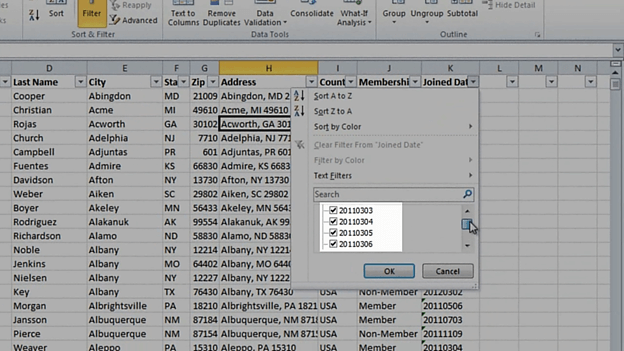
To convert the data type of this column into a date I’ll mark the entire range and then click [Convert] “Text to Columns”. I’ll leave the default options in the first step of the wizard, in the second step I’ll remove the space delimiter since we don’t have any and click next. Here in the third step of the wizard I get to set the data format. I’ll select “Date” and specify the format as Year, Month and Day (YMD) and then click “Finish”.

As you can see the format of the date has now been changed and if I click on the filter button I can select to filter on a specific year or month.
Closing (9:04)
I’m sure that you will quickly forget a lot of the steps I showed you in this video. Nevertheless, it’s important that you have seen it once so that you know it can be done automatically. You can always refer back to this video to remind yourself of the various steps. I’m Ulrika Hedlund for Business Productivity – thanks for watching!