How to change the layout of a pivot table in Excel 2010
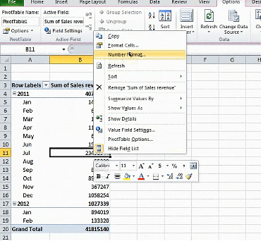
If I look at my Pivot Table I instantly get a good overview of the total sales for each month. To make this even easier to read I can change the number format and also the design of the PivotTable. First I’ll change the number format. To do that just right click and select Number format.

Here I’m going to select “Number”, use a [1000] comma separator and reduce the decimal places to zero.
The next thing I want to do is that I want to change how the PivotTable shows the subtotals.
Click the “Design” tab and then “Subtotals”. Here I’m going to select to “Show all Subtotals at Bottom of the Group”. So here you can see that for 2011 I get the 2011 total at the bottom and this is just a personal preference. I think it’s easier to see it this way.
Another thing I’d like to do is to add a blank row underneath each year. So I’ll click “Blank Rows” and select “Insert Blank Line after Each Item”. There, now there’s a clear distinction between each year.


![Use a [1000] comma separator and reduce the decimal places to zero How to change the layout of a PivotTable](http://businessproductivity.com/wp-content/uploads/2013/09/how-to-change-the-layout-of-a-pivottable-02.png)

